How to add a drop-down list to a Cell in Microsoft Excel

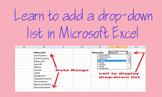
Learn to create a drop-down list to a cell in Excel. To add a list, we use the function of the data validation method to the given cell. We can edit, and remove lists to single and multiple selections.

In Microsoft Access you can limit a user to choose from the entries in the given set of data, in the same way, you can use this in other Office applications like Microsoft Excel by adding a drop-down list.

The main purpose of this feature is to give a user an option to choose an entry from the drop-down list instead of typing it. This feature is widely used, where we have multiple options for the users rather in the online data or in the office one, especially in the font color control or in the formatting toolbar.

Don’t Miss:

• Convert numbers into words in Excel in Indian and Pak Rupees
• Learn to Calculate Range in Excel for Given Set of Data

How to add a drop-down list in Excel:

In order to add an excel drop-down list to a cell, we use the simple technique and will generate it in minutes.

So follow the steps given below:

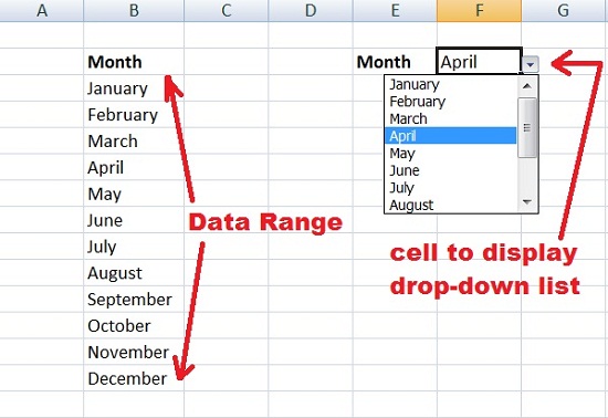
• Open a Microsoft Excel Sheet and Enter data in a column or in a row.
• Move the cursor to another cell to display a drop-down list.

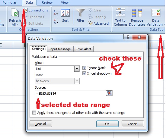
• Go to the Data tab, in the Data Tools group, and click Data Validation. ( Data tab>data tool group>data validation )
• The “data validation” dialog box will appear, in the Allow drop-down, Click List. (Also make sure to check both “ignore blank” and “in cell drop-down” options besides)
• Click the source box and select the data range and click ok.

• You can also type the items in the source box without selecting the data.

In this way, you can extend your data to multiple columns and rows.

Hope so you have got enough knowledge under discussion.

Note: in order to remove excel drop-down list, just go to the cell having the drop-down arrow and delete it.

Do comments with your feedback.

Watch the Video Tutorial below